Understanding LLMs from Scratch Utilizing Center College Math | by Rohit Patel | Oct, 2024

On this article, we discuss how Giant Language Fashions (LLMs) work, from scratch — assuming solely that you understand how so as to add and multiply two numbers. The article is supposed to be absolutely self-contained. We begin by constructing a easy Generative AI on pen and paper, after which stroll by every thing we have to have a agency understanding of recent LLMs and the Transformer structure. The article will strip out all the flowery language and jargon in ML and characterize every thing merely as they’re: numbers. We’ll nonetheless name out what issues are known as to tether your ideas while you learn jargon-y content material.

Going from addition/multiplication to essentially the most superior AI fashions at this time with out assuming different data or referring to different sources means we cowl a LOT of floor. That is NOT a toy LLM clarification — a decided particular person can theoretically recreate a contemporary LLM from all the knowledge right here. I’ve lower out each phrase/line that was pointless and as such this text isn’t actually meant to be browsed.

1. A easy neural community
2. How are these fashions educated?
3. How does all this generate language?
4. What makes LLMs work so properly?
5. Embeddings
6. Sub-word tokenizers
7. Self-attention
8. Softmax
9. Residual connections
10. Layer Normalization
11. Dropout
12. Multi-head consideration
13. Positional embeddings
14. The GPT structure
15. The transformer structure

Let’s dive in.

The very first thing to notice is that neural networks can solely take numbers as inputs and output different numbers. No exceptions. The artwork is in determining how one can feed your inputs as numbers, deciphering the output numbers in a means that achieves your targets. And eventually, constructing neural nets that can take the inputs you present and provide the outputs you need (given the interpretation you selected for these outputs). Let’s stroll by how we get from including and multiplying numbers to issues like Llama 3.1.

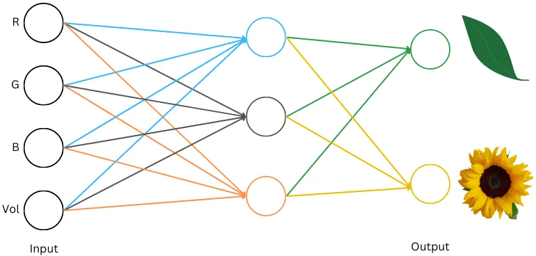
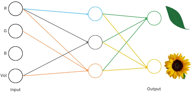
Let’s work by a easy neural community that may classify an object:

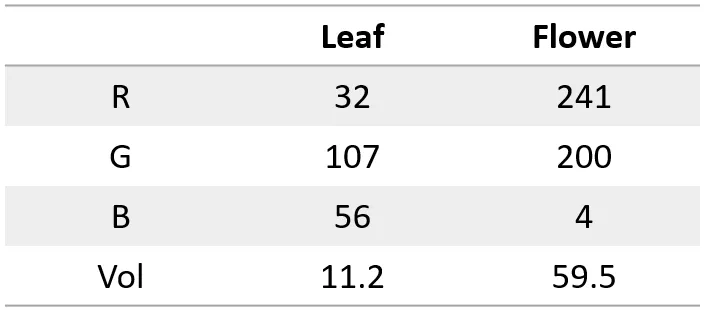
• Object knowledge obtainable: Dominant colour (RGB) & Quantity (in milli-liters)
• Classify into: Leaf OR Flower

Right here’s what the information for a leaf and a sunflower can appear like:

Let’s now construct a neural internet that does this classification. We have to determine on enter/output interpretations. Our inputs are already numbers, so we are able to feed them immediately into the community. Our outputs are two objects, leaf and flower which the neural community can’t output. Let’s take a look at a few schemes we are able to use right here:

• We will make the community output a single quantity. And if the quantity is constructive we are saying it’s a leaf and whether it is destructive we are saying it’s a flower
• OR, we are able to make the community output two numbers. We interpret the primary one as a quantity for leaf and second one because the quantity for flower and we are going to say that the choice is whichever quantity is bigger

Each schemes permit the community to output quantity(s) that we are able to interpret as leaf or flower. Let’s decide the second scheme right here as a result of it generalizes properly to different issues we are going to take a look at later. And right here’s a neural community that does the classification utilizing this scheme. Let’s work by it:

Blue circle like so: (32 * 0.10) + (107 * -0.29) + (56 * -0.07) + (11.2 * 0.46) = — 26.6

Some jargon:

Neurons/nodes: The numbers within the circles

Weights: The coloured numbers on the traces

Layers: A set of neurons known as a layer. You could possibly consider this community as having 3 layers: Enter layer with 4 neurons, Center layer with 3 neurons, and the Output layer with 2 neurons.

To calculate the prediction/output from this community (known as a “ahead cross”), you begin from the left. Now we have the information obtainable for the neurons within the Enter layer. To maneuver “ahead” to the following layer, you multiply the quantity within the circle with the burden for the corresponding neuron pairing and also you add all of them up. We show blue and orange circle math above. Operating the entire community we see that the primary quantity within the output layer comes out increased so we interpret it as “community categorized these (RGB,Vol) values as leaf”. A properly educated community can take numerous inputs for (RGB,Vol) and accurately classify the article.

The mannequin has no notion of what a leaf or a flower is, or what (RGB,Vol) are. It has a job of taking in precisely 4 numbers and giving out precisely 2 numbers. It’s our interpretation that the 4 enter numbers are (RGB,Vol) and it is usually our resolution to have a look at the output numbers and infer that if the primary quantity is bigger it’s a leaf and so forth. And eventually, it is usually as much as us to decide on the correct weights such that the mannequin will take our enter numbers and provides us the correct two numbers such that after we interpret them we get the interpretation we would like.

An attention-grabbing aspect impact of that is that you would be able to take the identical community and as a substitute of feeding RGB,Vol feed different 4 numbers like cloud cowl, humidity and so on.. and interpret the 2 numbers as “Sunny in an hour” or “Wet in an hour” after which if in case you have the weights properly calibrated you will get the very same community to do two issues on the identical time — classify leaf/flower and predict rain in an hour! The community simply provides you two numbers, whether or not you interpret it as classification or prediction or one thing else is fully as much as you.

Stuff omitted for simplification (be happy to disregard with out compromising comprehensibility):

• Activation layer: A vital factor lacking from this community is an “activation layer”. That’s a flowery phrase for saying that we take the quantity in every circle and apply a nonlinear perform to it (RELU is a typical perform the place you simply take the quantity and set it to zero whether it is destructive, and go away it unchanged whether it is constructive). So mainly in our case above, we might take the center layer and change the 2 numbers (-26.6 and -47.1) with zeros earlier than we proceed additional to the following layer. In fact, we must re-train the weights right here to make the community helpful once more. With out the activation layer all of the additions and multiplications within the community could be collapsed to a single layer. In our case, you may write the inexperienced circle because the sum of RGB immediately with some weights and you wouldn’t want the center layer. It could be one thing like (0.10 * -0.17 + 0.12 * 0.39–0.36 * 0.1) * R + (-0.29 * -0.17–0.05 * 0.39–0.21 * 0.1) * G …and so forth. That is often not attainable if now we have a nonlinearity there. This helps networks take care of extra advanced conditions.
• Bias: Networks will often additionally include one other quantity related to every node, this quantity is just added to the product to calculate the worth of the node and this quantity known as the “bias”. So if the bias for the highest blue node was 0.25 then the worth within the node could be: (32 * 0.10) + (107 * -0.29) + (56 * -0.07) + (11.2 * 0.46) + 0.25 = — 26.35. The phrase parameters is often used to check with all these numbers within the mannequin that aren’t neurons/nodes.
• Softmax: We don’t often interpret the output layer immediately as proven in our fashions. We convert the numbers into chances (i.e. make it so that each one numbers are constructive and add as much as 1). If all of the numbers within the output layer had been already constructive a method you may obtain that is by dividing every quantity by the sum of all numbers within the output layer. Although a “softmax” perform is often used which might deal with each constructive and destructive numbers.

Within the instance above, we magically had the weights that allowed us to place knowledge into the mannequin and get output. However how are these weights decided? The method of setting these weights (or “parameters”) known as “coaching the mannequin”, and we want some coaching knowledge to coach the mannequin.

Let’s say now we have some knowledge the place now we have the inputs and we already know if every enter corresponds to leaf or flower, that is our “coaching knowledge” and since now we have the leaf/flower label for every set of (R,G,B,Vol) numbers, that is “labeled knowledge”.

Right here’s the way it works:

• Begin with a random numbers, i.e. set every parameter/weight to a random quantity
• Now, we all know that after we enter the information similar to the leaf (R=32, G=107, B=56, Vol=11.2). Suppose we would like a bigger quantity for leaf within the output layer. Let’s say we would like the quantity similar to leaf as 0.8 and the one similar to flower as 0.2 (as proven in instance above, however these are illustrative numbers to show coaching, in actuality we might not need 0.8 and 0.2. In actuality these could be chances, which they aren’t right here, and we’d them to be 1 and 0)
• We all know the numbers we would like within the output layer, and the numbers we’re getting from the randomly chosen parameters (that are totally different from what we would like). So for all of the neurons within the output layer, let’s take the distinction between the quantity we would like and the quantity now we have. Then add up the variations. E.g., if the output layer is 0.6 and 0.4 within the two neurons, then we get: (0.8–0.6)=0.2 and (0.2–0.4)= -0.2 so we get a complete of 0.4 (ignoring minus indicators earlier than including). We will name this our “loss”. Ideally we would like the loss to be near zero, i.e. we need to “decrease the loss”.
• As soon as now we have the loss, we are able to barely change every parameter to see if growing or reducing it’s going to improve the loss or lower it. That is known as the “gradient” of that parameter. Then we are able to transfer every of the parameters by a small quantity within the path the place the loss goes down (the path of the gradient). As soon as now we have moved all of the parameters barely, the loss needs to be decrease
• Preserve repeating the method and you’ll cut back the loss, and ultimately have a set of weights/parameters which can be “educated”. This complete course of known as “gradient descent”.

Couple of notes:

• You usually have a number of coaching examples, so while you change the weights barely to attenuate the loss for one instance it’d make the loss worse for one more instance. The best way to take care of that is to outline loss as common loss over all of the examples after which take gradient over that common loss. This reduces the typical loss over your entire coaching knowledge set. Every such cycle known as an “epoch”. Then you may hold repeating the epochs thus discovering weights that cut back common loss.
• We don’t truly must “transfer weights round” to calculate the gradient for every weight — we are able to simply infer it from the method (e.g. if the burden is 0.17 within the final step, and the worth of neuron is constructive, and we would like a bigger quantity in output we are able to see that growing this quantity to 0.18 will assist).

In apply, coaching deep networks is a tough and sophisticated course of as a result of gradients can simply spiral uncontrolled, going to zero or infinity throughout coaching (known as “vanishing gradient” and “exploding gradient” issues). The straightforward definition of loss that we talked about right here is completely legitimate, however not often used as there are higher practical types that work properly for particular functions. With trendy fashions containing billions of parameters, coaching a mannequin requires large compute assets which has its personal issues (reminiscence limitations, parallelization and so on.)

Bear in mind, neural nets absorb some numbers, do some math primarily based on the educated parameters, and provides out another numbers. Every little thing is about interpretation and coaching the parameters (i.e. setting them to some numbers). If we are able to interpret the 2 numbers as “leaf/flower” or “rain or solar in an hour”, we are able to additionally interpret them as “subsequent character in a sentence”.

However there are greater than 2 letters in English, and so we should develop the variety of neurons within the output layer to, say, the 26 letters within the English language (let’s additionally throw in some symbols like house, interval and so on..). Every neuron can correspond to a personality and we take a look at the (26 or so) neurons within the output layer and say that the character similar to the very best numbered neuron within the output layer is the output character. Now now we have a community that may take some inputs and output a personality.

What if we change the enter in our community with these characters: “Humpty Dumpt” and requested it to output a personality and interpreted it because the “Community’s suggestion of the following character within the sequence that we simply entered”. We will in all probability set the weights properly sufficient for it to output “y” — thereby finishing “Humpty Dumpty”. Apart from one downside, how will we enter these lists of characters within the community? Our community solely accepts numbers!!

One easy resolution is to assign a quantity to every character. Let’s say a=1, b=2 and so forth. Now we are able to enter “humpty dumpt” and practice it to provide us “y”. Our community appears one thing like this:

Okay, so now we are able to predict one character forward by offering the community an inventory of characters. We will use this truth to construct a complete sentence. For instance, as soon as now we have the “y” predicted, we are able to append that “y” to the record of characters now we have and feed it to the community and ask it to foretell the following character. And if properly educated it ought to give us an area, and so forth and so forth. By the tip, we must always be capable of recursively generate “Humpty Dumpty sat on a wall”. Now we have Generative AI. Furthermore, we now have a community able to producing language! Now, no one ever truly places in randomly assigned numbers and we are going to see extra wise schemes down the road. Should you can’t wait, be happy to take a look at the one-hot encoding part within the appendix.

Astute readers will observe that we are able to’t truly enter “Humpty Dumpty” into the community because the means the diagram is, it solely has 12 neurons within the enter layer one for every character in “humpty dumpt” (together with the house). So how can we put within the “y” for the following cross. Placing a thirteenth neuron there would require us to switch your entire community, that’s not workable. The answer is straightforward, let’s kick the “h” out and ship the 12 most up-to-date characters. So we might be sending “umpty dumpty” and the community will predict an area. Then we might enter “mpty dumpty “ and it’ll produce an s and so forth. It appears one thing like this:

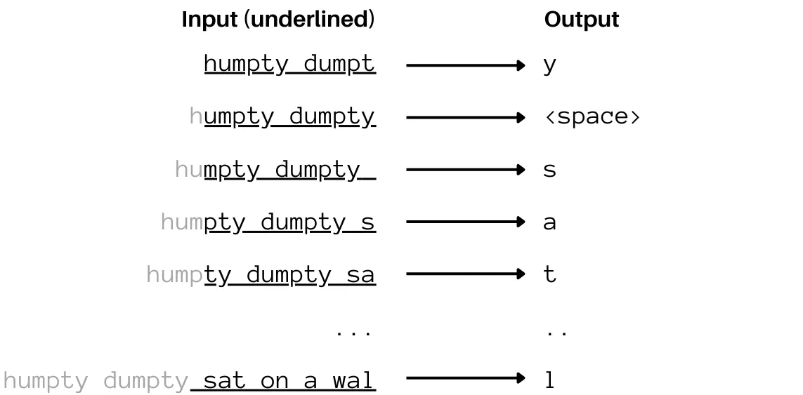
We’re throwing away a variety of info within the final line by feeding the mannequin solely “ sat on the wal”. So what do the newest and best networks of at this time do? Kind of precisely that. The size of inputs we are able to put right into a community is fastened (decided by the dimensions of the enter layer). That is known as “context size” — the context that’s offered to the community to make future predictions. Trendy networks can have very giant context lengths (a number of thousand phrases) and that helps. There are some methods of inputting infinite size sequences however the efficiency of these strategies, whereas spectacular, has since been surpassed by different fashions with giant (however fastened) context size.

One different factor cautious readers will discover is that now we have totally different interpretations for inputs and outputs for a similar letters! For instance, when inputting “h” we’re merely denoting it with the quantity 8 however on the output layer we’re not asking the mannequin to output a single quantity (8 for “h”, 9 for “i” and so forth..) as a substitute we’re are asking the mannequin to output 26 numbers after which we see which one is the very best after which if the eighth quantity is highest we interpret the output as “h”. Why don’t we use the identical, constant, interpretation on each ends? We may, it’s simply that within the case of language, liberating your self to decide on between totally different interpretations provides you a greater likelihood of constructing higher fashions. And it simply so occurs that the simplest presently recognized interpretations for the enter and output are totally different. In-fact, the way in which we’re inputting numbers on this mannequin just isn’t one of the best ways to do it, we are going to take a look at higher methods to try this shortly.

Producing “Humpty Dumpty sat on a wall” character-by-character is a far cry from what trendy LLMs can do. There are a selection of variations and improvements that get us from the straightforward generative AI that we mentioned above to the human-like bot. Let’s undergo them:

Bear in mind we stated that the way in which that we’re inputting characters into the mannequin isn’t one of the best ways to do it. We simply arbitrarily chosen a quantity for every character. What if there have been higher numbers we may assign that may make it attainable for us to coach higher networks? How do we discover these higher numbers? Right here’s a intelligent trick:

Once we educated the fashions above, the way in which we did it was by shifting round weights and seeing that provides us a smaller loss ultimately. After which slowly and recursively altering the weights. At every flip we might:

• Feed within the inputs
• Calculate the output layer
• Evaluate it to the output we ideally need and calculate the typical loss
• Alter the weights and begin once more

On this course of, the inputs are fastened. This made sense when inputs had been (RGB, Vol). However the numbers we’re placing in now for a,b,c and so on.. are arbitrarily picked by us. What if at each iteration along with shifting the weights round by a bit we additionally moved the enter round and see if we are able to get a decrease loss through the use of a distinct quantity to characterize “a” and so forth? We’re positively lowering the loss and making the mannequin higher (that’s the path we moved a’s enter in, by design). Principally, apply gradient descent not simply to the weights but additionally the quantity representations for the inputs since they’re arbitrarily picked numbers anyway. That is known as an “embedding”. It’s a mapping of inputs to numbers, and as you simply noticed, it must be educated. The method of coaching an embedding is very similar to that of coaching a parameter. One large benefit of this although is that after you practice an embedding you should utilize it in one other mannequin if you want. Remember the fact that you’ll persistently use the identical embedding to characterize a single token/character/phrase.

We talked about embeddings which can be only one quantity per character. Nevertheless, in actuality embeddings have a couple of quantity. That’s as a result of it’s laborious to seize the richness of idea by a single quantity. If we take a look at our leaf and flower instance, now we have 4 numbers for every object (the dimensions of the enter layer). Every of those 4 numbers conveyed a property and the mannequin was ready to make use of all of them to successfully guess the article. If we had just one quantity, say the pink channel of the colour, it may need been rather a lot tougher for the mannequin. We’re attempting to seize human language right here — we’re going to wish a couple of quantity.

So as a substitute of representing every character by a single quantity, possibly we are able to characterize it by a number of numbers to seize the richness? Let’s assign a bunch of numbers to every character. Let’s name an ordered assortment of numbers a “vector” (ordered as in every quantity has a place, and if we swap place of two numbers it provides us a distinct vector. This was the case with our leaf/flower knowledge, if we swapped the R and G numbers for the leaf, we might get a distinct colour, it will not be the identical vector anymore). The size of a vector is just what number of numbers it incorporates. We’ll assign a vector to every character. Two questions come up:

• If now we have a vector assigned to every character as a substitute of a quantity, how will we now feed “humpty dumpt” to the community? The reply is straightforward. Let’s say we assigned a vector of 10 numbers to every character. Then as a substitute of the enter layer having 12 neurons we might simply put 120 neurons there since every of the 12 characters in “humpty dumpt” has 10 numbers to enter. Now we simply put the neurons subsequent to one another and we’re good to go
• How do we discover these vectors? Fortunately, we simply realized how one can practice embedding numbers. Coaching an embedding vector isn’t any totally different. You now have 120 inputs as a substitute of 12 however all you’re doing is shifting them round to see how one can decrease loss. And then you definately take the primary 10 of these and that’s the vector similar to “h” and so forth.

All of the embedding vectors should after all be the identical size, in any other case we might not have a means of coming into all of the character combos into the community. E.g. “humpty dumpt” and within the subsequent iteration “umpty dumpty” — in each instances we’re coming into 12 characters within the community and if every of the 12 characters was not represented by vectors of size 10 we received’t be capable of reliably feed all of them right into a 120-long enter layer. Let’s visualize these embedding vectors:

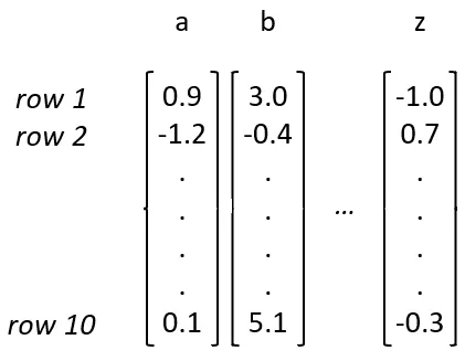
Let’s name an ordered assortment of same-sized vectors a matrix. This matrix above known as an embedding matrix. You inform it a column quantity similar to your letter and that column within the matrix will provide you with the vector that you’re utilizing to characterize that letter. This may be utilized extra typically for embedding any arbitrary assortment of issues — you’d simply must have as many columns on this matrix because the issues you’ve.

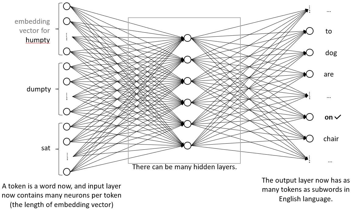
To date, now we have been working with characters as the fundamental constructing blocks of language. This has its limitations. The neural community weights must do a variety of the heavy lifting the place they have to make sense of sure sequences of characters (i.e. phrases) showing subsequent to one another after which subsequent to different phrases. What if we immediately assigned embeddings to phrases and made the community predict the following phrase. The community doesn’t perceive something greater than numbers anyway, so we are able to assign a 10-length vector to every of the phrases “humpty”, “dumpty”, “sat”, “on” and so on.. after which we simply feed it two phrases and it may give us the following phrase. “Token” is the time period for a single unit that we embed after which feed to the mannequin. Our fashions to this point had been utilizing characters as tokens, now we’re proposing to make use of whole phrases as a token (you may after all use whole sentences or phrases as tokens when you like).

Utilizing phrase tokenization has one profound impact on our mannequin. There are greater than 180K phrases within the English language. Utilizing our output interpretation scheme of getting a neuron per attainable output we want tons of of hundreds of neurons within the output layer insead of the 26 or so. With the dimensions of the hidden layers wanted to realize significant outcomes for contemporary networks, this subject turns into much less urgent. What’s nevertheless value noting is that since we’re treating every phrase individually, and we’re beginning with a random quantity embeddings for every — very comparable phrases (e.g. “cat” and “cats”) will begin with no relationship. You’d anticipate that embeddings for the 2 phrases needs to be shut to one another — which undoubtedly the mannequin will be taught. However, can we someway use this apparent similarity to get a jumpstart and simplify issues?

Sure we are able to. The commonest embedding scheme in language fashions at this time is one thing the place you break phrases down into subwords after which embed them. Within the cat instance, we might break down cats into two tokens “cat” and ”s”. Now it’s simpler for the mannequin to know the idea of “s” adopted by different acquainted phrases and so forth. This additionally reduces the variety of tokens we want (sentencpiece is a typical tokenizer with vocab measurement choices in tens of hundreds vs tons of of hundreds of phrases in english). A tokenizer is one thing that takes you enter textual content (e.g. “Humpty Dumpt”) and splits it into the tokens and offers you the corresponding numbers that you have to search for the embedding vector for that token within the embedding matrix. For instance, in case of “humpty dumpty” if we’re utilizing character degree tokenizer and we organized our embedding matrix as within the image above, then the tokenizer will first cut up humpty dumpt into characters [‘h’,’u’,…’t’] after which offer you again the numbers [8,21,…20] as a result of you have to search for the eighth column of the embedding matrix to get the embedding vector for ‘h’ (embedding vector is what you’ll feed into the mannequin, not the quantity 8, in contrast to earlier than). The association of the columns within the matrix is totally irrelevant, we may assign any column to ‘h’ and so long as we glance up the identical vector each time we enter ‘h’ we needs to be good. Tokenizers simply give us an arbitrary (however fastened) quantity to make lookup simple. The primary activity we want them for actually is splitting the sentence in tokens.

With embeddings and subword tokenization, a mannequin may look one thing like this:

The subsequent few sections take care of more moderen advances in language modeling, and those that made LLMs as highly effective as they’re at this time. Nevertheless, to know these there are just a few fundamental math ideas you have to know. Listed below are the ideas:

• Matrices and matrix multiplication
• Normal idea of capabilities in arithmetic
• Elevating numbers to powers (e.g. a3 = a*a*a)
• Pattern imply, variance, and customary deviation

I’ve added summaries of those ideas within the appendix.

To date now we have seen just one easy neural community construction (known as feedforward community), one which incorporates a variety of layers and every layer is absolutely linked to the following (i.e., there’s a line connecting any two neurons in consecutive layers), and it is just linked to the following layer (e.g. no traces between layer 1 and layer 3 and so on..). Nevertheless, as you may think about there may be nothing stopping us from eradicating or making different connections. And even making extra advanced buildings. Let’s discover a very essential construction: self-attention.

Should you take a look at the construction of human language, the following phrase that we need to predict will rely on all of the phrases earlier than. Nevertheless, they might rely on some phrases earlier than them to a larger diploma than others. For instance, if we are attempting to foretell the following phrase in “Damian had a secret little one, a lady, and he had written in his will that each one his belongings, together with the magical orb, will belong to ____”. This phrase right here might be “her” or “his” and it relies upon particularly on a a lot earlier phrase within the sentence: lady/boy.

The excellent news is, our easy feedforward mannequin connects to all of the phrases within the context, and so it may be taught the suitable weights for essential phrases, However right here’s the issue, the weights connecting particular positions in our mannequin by feed ahead layers are fastened (for each place). If the essential phrase was all the time in the identical place, it will be taught the weights appropriately and we’d be nice. Nevertheless, the related phrase to the following prediction might be anyplace within the system. We may paraphrase that sentence above and when guessing “her vs his”, one crucial phrase for this prediction could be boy/lady irrespective of the place it appeared in that sentence. So, we want weights that rely not solely on the place but additionally on the content material in that place. How will we obtain this?

Self consideration does one thing like including up the embedding vectors for every of the phrases, however as a substitute of immediately including them up it applies some weights to every. So if the embedding vectors for humpty,dumpty, sat are x1, x2, x3 respectively, then it’s going to multiply every one with a weight (a quantity) earlier than including them up. One thing like output = 0.5 x1 + 0.25 x2 + 0.25 x3 the place output is the self-attention output. If we write the weights as u1, u2, u3 such that output = u1x1+u2x2+u3x3 then how do we discover these weights u1, u2, u3?

Ideally, we would like these weights to be depending on the vector we’re including — as we noticed some could also be extra essential than others. However essential to whom? To the phrase we’re about to foretell. So we additionally need the weights to rely on the phrase we’re about to foretell. Now that’s a difficulty, we after all don’t know the phrase we’re about to foretell earlier than we predict it. So, self consideration makes use of the phrase instantly previous the phrase we’re about to foretell, i.e., the final phrase within the sentence obtainable (I don’t actually know why this and why not one thing else, however a variety of issues in deep studying are trial and error and I believe this works properly).

Nice, so we would like weights for these vectors, and we would like every weight to rely on the phrase that we’re aggregating and phrase instantly previous the one we’re going to predict. Principally, we would like a perform u1 = F(x1, x3) the place x1 is the phrase we are going to weight and x3 is the final phrase within the sequence now we have (assuming now we have solely 3 phrases). Now, an easy means of attaining that is to have a vector for x1 (let’s name it k1) and a separate vector for x3 (let’s name it q3) after which merely take their dot product. This may give us a quantity and it’ll rely on each x1 and x3. How will we get these vectors k1 and q3? We construct a tiny single layer neural community to go from x1 to k1 (or x2 to k2, x3 to k3 and so forth). And we construct one other community going from x3 to q3 and so on… Utilizing our matrix notation, we mainly provide you with weight matrices Wk and Wq such that k1 = Wkx1 and q1 =Wqx1 and so forth. Now we are able to take a dot product of k1 and q3 to get a scalar, so u1 = F(x1,x3) = Wkx1 · Wqx3.

One further factor that occurs in self-attention is that we don’t immediately take the weighted sum of the embedding vectors themselves. As an alternative, we take the weighted sum of some “worth” of that embedding vector, which is obtained by one other small single layer community. What this implies is much like k1 and q1, we additionally now have a v1 for the phrase x1 and we receive it by a matrix Wv such that v1=Wvx1. This v1 is then aggregated. So all of it appears one thing like this if we solely have 3 phrases and we are attempting to foretell the fourth:

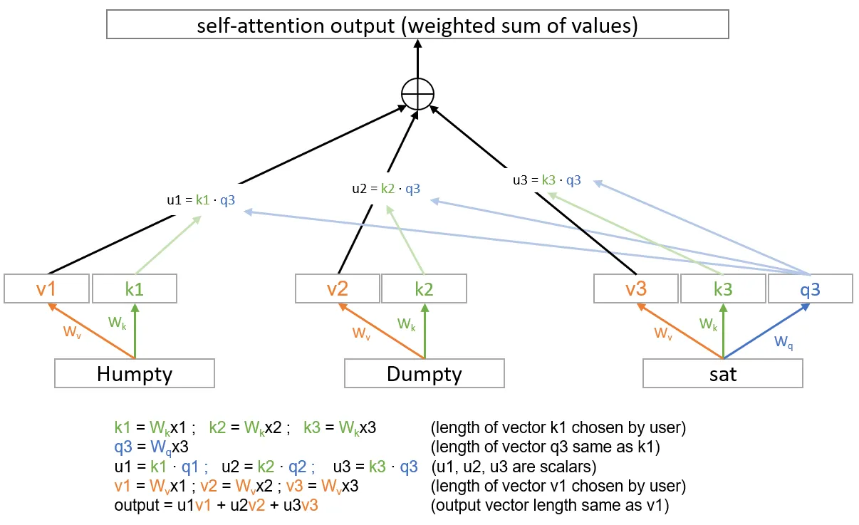
The plus signal represents a easy addition of the vectors, implying they must have the identical size. One final modification not proven right here is that the scalars u1, u2, u3 and so on.. received’t essentially add as much as 1. If we want them to be weights, we must always make them add up. So we are going to apply a well-recognized trick right here and use the softmax perform.

That is self-attention. There may be additionally cross-attention the place you may have the q3 come from the final phrase, however the okay’s and the v’s can come from one other sentence altogether. That is for instance precious in translation duties. Now we all know what consideration is.

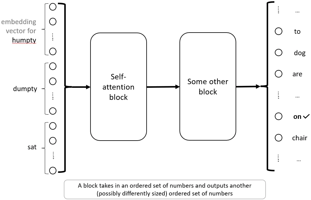
This complete factor can now be put in a field and be known as a “self consideration block”. Principally, this self consideration block takes within the embedding vectors and spits out a single output vector of any user-chosen size. This block has three parameters, Wk,Wq,Wv — it doesn’t should be extra difficult than that. There are numerous such blocks within the machine studying literature, and they’re often represented by bins in diagrams with their title on it. One thing like this:

One of many issues that you’ll discover with self-attention is that the place of issues to this point doesn’t appear related. We’re utilizing the identical W’s throughout the board and so switching Humpty and Dumpty received’t actually make a distinction right here — all numbers will find yourself being the identical. Which means whereas consideration can determine what to concentrate to, this received’t rely on phrase place. Nevertheless, we do know that phrase positions are essential in english and we are able to in all probability enhance efficiency by giving the mannequin some sense of a phrase’s place.

And so, when consideration is used, we don’t usually feed the embedding vectors on to the self consideration block. We’ll later see how “positional encoding” is added to embedding vectors earlier than feeding to consideration blocks.

Notice for the pre-initiated: These for whom this isn’t the primary time studying about self-attention will observe that we’re not referencing any Okay and Q matrices, or making use of masks and so on.. That’s as a result of these issues are implementation particulars arising out of how these fashions are generally educated. A batch of knowledge is fed and the mannequin is concurrently educated to foretell dumpty from humpty, sat from humpty dumpty and so forth. It is a matter of gaining effectivity and doesn’t have an effect on interpretation and even mannequin outputs, and now we have chosen to omit coaching effectivity hacks right here.

We talked briefly about softmax within the very first observe. Right here’s the issue softmax is attempting to resolve: In our output interpretation now we have as many neurons because the choices from which we would like the community to pick out one. And we stated that we’re going to interpret the community’s selection as the very best worth neuron. Then we stated we’re going to calculate loss because the distinction between the worth that community gives, and a great worth we would like. However what’s that perfect worth we would like? We set it to 0.8 within the leaf/flower instance. However why 0.8? Why no 5, or 10, or 10 million? The upper the higher for that coaching instance. Ideally we would like infinity there! Now that may make the issue intractable — all loss could be infinite and our plan of minimizing loss by shifting round parameters (keep in mind “gradient descent”) fails. How will we take care of this?

One easy factor we are able to do is cap the values we would like. Let’s say between 0 and 1? This may make all loss finite, however now now we have the problem of what occurs when the community overshoots. Let’s say it outputs (5,1) for (leaf,flower) in a single case, and (0,1) in one other. The primary case made the correct selection however the loss is worse! Okay, so now we want a solution to additionally convert the outputs of the final layer in (0,1) vary in order that it preserves the order. We may use any perform (a “perform” in arithmetic is just a mapping of 1 quantity to a different — in goes one quantity, out comes one other — it’s rule primarily based by way of what will likely be output for a given enter) right here to get the job completed. One attainable choice is the logistic perform (see graph beneath) which maps all numbers to numbers between (0,1) and preserves the order:

Now, now we have a quantity between 0 and 1 for every of the neurons within the final layer and we are able to calculate loss by setting the right neuron to 1, others to 0 and taking the distinction of that from what the community gives us. This may work, however can we do higher?

Going again to our “Humpty dumpty” instance, let’s say we are attempting to generate dumpty character-by-character and our mannequin makes a mistake when predicting “m” in dumpty. As an alternative of giving us the final layer with “m” as the very best worth, it provides us “u” as the very best worth however “m” is an in depth second.

Now we are able to proceed with “duu” and attempt to predict subsequent character and so forth, however the mannequin confidence will likely be low as a result of there aren’t that many good continuations from “humpty duu..”. Then again, “m” was an in depth second, so we are able to additionally give “m” a shot, predict the following few characters, and see what occurs? Possibly it provides us a greater total phrase?

So what we’re speaking about right here is not only blindly deciding on the max worth, however attempting just a few. What’s a great way to do it? Effectively now we have to assign an opportunity to every one — say we are going to decide the highest one with 50%, second one with 25% and so forth. That’s a great way to do it. However possibly we might need the prospect to be depending on the underlying mannequin predictions. If the mannequin predicts values for m and u to be actually shut to one another right here (in comparison with different values) — then possibly an in depth 50–50 likelihood of exploring the 2 is a good suggestion?

So we want a pleasant rule that takes all these numbers and converts them into possibilities. That’s what softmax does. It’s a generalization of the logistic perform above however with further options. Should you give it 10 arbitrary numbers — it will provide you with 10 outputs, every between 0 and 1 and importantly, all 10 including as much as 1 in order that we are able to interpret them as likelihood. You will see that softmax because the final layer in practically each language mannequin.

Now we have slowly modified our visualization of networks because the sections progress. We at the moment are utilizing bins/blocks to indicate sure ideas. This notation is beneficial in denoting a very helpful idea of residual connections. Let’s take a look at residual connection mixed with a self-attention block:

Notice that we put “Enter” and “Output” as bins to make issues less complicated, however these are nonetheless mainly only a assortment of neurons/numbers identical as proven above.

So what’s happening right here? We’re mainly taking the output of self-attention block and earlier than passing it to the following block, we’re including to it the unique Enter. Very first thing to notice is that this is able to require that the size of the self-attention block output should now be the identical as that of the enter. This isn’t an issue since as we famous the self-attention output is decided by the consumer. However why do that? We received’t get into all the main points right here however the important thing factor is that as networks get deeper (extra layers between enter and output) it will get more and more tougher to coach them. Residual connections have been proven to assist with these coaching challenges.

Layer normalization is a reasonably easy layer that takes the information coming into the layer and normalizes it by subtracting the imply and dividing it by customary deviation (possibly a bit extra, as we see beneath). For instance, if we had been to use layer normalization instantly after the enter, it will take all of the neurons within the enter layer after which it will calculate two statistics: their imply and their customary deviation. Let’s say the imply is M and the usual deviation is S then what layer norm is doing is taking every of those neurons and changing it with (x-M)/S the place x denotes any given neuron’s authentic worth.

Now how does this assist? It mainly stabilizes the enter vector and helps with coaching deep networks. One concern is that by normalizing inputs, are we eradicating some helpful info from them that could be useful in studying one thing precious about our purpose? To deal with this, the layer norm layer has a scale and a bias parameter. Principally, for every neuron you simply multiply it with a scalar after which add a bias to it. These scalar and bias values are parameters that may be educated. This permits the community to be taught a number of the variation that could be precious to the predictions. And since these are the one parameters, the LayerNorm block doesn’t have a variety of parameters to coach. The entire thing appears one thing like this:

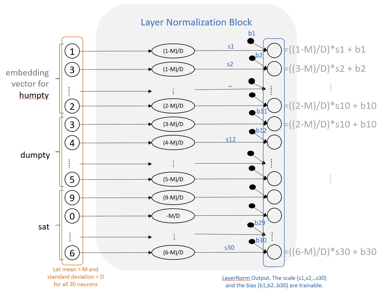
The Scale and Bias are trainable parameters. You may see that layer norm is a comparatively easy block the place every quantity is barely operated on pointwise (after the preliminary imply and std calculation). Reminds us of the activation layer (e.g. RELU) with the important thing distinction being that right here now we have some trainable parameters (albeit lot fewer than different layers due to the straightforward pointwise operation).

Normal deviation is a statistical measure of how unfold out the values are, e.g., if the values are all the identical you’d say the usual deviation is zero. If, on the whole, every worth is de facto removed from the imply of those exact same values, then you’ll have a excessive customary deviation. The method to calculate customary deviation for a set of numbers, a1, a2, a3…. (say N numbers) goes one thing like this: subtract the imply (of those numbers) from every of the numbers, then sq. the reply for every of N numbers. Add up all these numbers after which divide by N. Now take a sq. root of the reply.

Notice for the pre-initiated: Skilled ML professionals will observe that there is no such thing as a dialogue of batch norm right here. In-fact, we haven’t even launched the idea of batches on this article in any respect. For essentially the most half, I consider batches are one other coaching accelerant not associated to the understanding of core ideas (besides maybe batch norm which we don’t want right here).

Dropout is an easy however efficient technique to keep away from mannequin overfitting. Overfitting is a time period for while you practice the mannequin in your coaching knowledge, and it really works properly on that dataset however doesn’t generalize properly to the examples the mannequin has not seen. Strategies that assist us keep away from overfitting are known as “regularization methods”, and dropout is one among them.

Should you practice a mannequin, it’d make errors on the information and/or overfit it in a specific means. Should you practice one other mannequin, it’d do the identical, however otherwise. What when you educated a variety of these fashions and averaged the outputs? These are sometimes known as “ensemble fashions” as a result of they predict the outputs by combining outputs from an ensemble of fashions, and ensemble fashions typically carry out higher than any of the person fashions.

In neural networks, you may do the identical. You could possibly construct a number of (barely totally different) fashions after which mix their outputs to get a greater mannequin. Nevertheless, this may be computationally costly. Dropout is a method that doesn’t fairly construct ensemble fashions however does seize a number of the essence of the idea.

The idea is straightforward, by inserting a dropout layer throughout coaching what you’re doing is randomly deleting a sure proportion of the direct neuron connections between the layers that dropout is inserted. Contemplating our preliminary community and inserting a Dropout layer between the enter and the center layer with 50% dropout fee can look one thing like this:

Now, this forces the community to coach with a variety of redundancy. Basically, you’re coaching a variety of totally different fashions on the identical time — however they share weights.

Now for making inferences, we may comply with the identical strategy as an ensemble mannequin. We may make a number of predictions utilizing dropouts after which mix them. Nevertheless, since that’s computationally intensive — and since our fashions share frequent weights — why don’t we simply do a prediction utilizing all of the weights (so as a substitute of utilizing 50% of the weights at a time we use all on the identical time). This could give us some approximation of what an ensemble will present.

One subject although: the mannequin educated with 50% of the weights could have very totally different numbers within the center neurons than one utilizing all of the weights. What we would like is extra ensemble type averaging right here. How will we do that? Effectively, a easy means is to easily take all of the weights and multiply them by 0.5 since we at the moment are utilizing twice as many weights. That is what Droput does throughout inference. It’ll use the complete community with all of the weights and easily multiply the weights with (1- p) the place p is the deletion likelihood. And this has been proven to work relatively properly as a regularization approach.

That is the important thing block within the transformer structure. We’ve already seen what an consideration block is. Do not forget that the output of an consideration block was decided by the consumer and it was the size of v’s. What a multi-attention head is mainly you run a number of consideration heads in parallel (all of them take the identical inputs). Then we take all their outputs and easily concatenate them. It appears one thing like this:

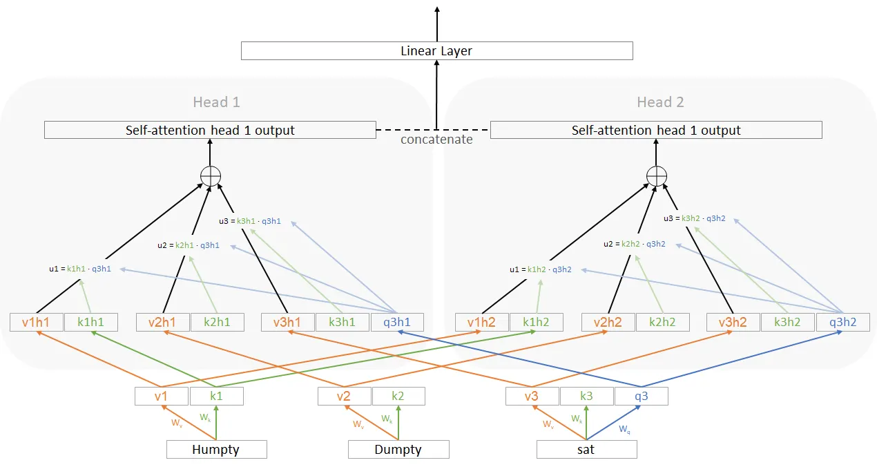
Bear in mind the arrows going from v1 -> v1h1 are linear layers — there’s a matrix on every arrow that transforms. I simply didn’t present them to keep away from litter.

What’s going on right here is that we’re producing the identical key, question and values for every of the heads. However then we’re mainly making use of a linear transformation on prime of that (individually to every okay,q,v and individually for every head) earlier than we use these okay,q,v values. This additional layer didn’t exist in self consideration.

A aspect observe is that to me, this can be a barely stunning means of making a multi-headed consideration. For instance, why not create separate Wk,Wq,Wv matrices for every of the heads relatively than including a brand new layer and sharing these weights. Let me know if — I actually don’t know.

We briefly talked concerning the motivation for utilizing positional encoding within the self-attention part. What are these? Whereas the image reveals positional encoding, utilizing a positional embedding is extra frequent than utilizing an encoding. As such we discuss a typical positional embedding right here however the appendix additionally covers positional encoding used within the authentic paper. A positional embedding isn’t any totally different than some other embedding besides that as a substitute of embedding the phrase vocabulary we are going to embed numbers 1, 2, 3 and so on. So this embedding is a matrix of the identical size as phrase embedding, and every column corresponds to a quantity. That’s actually all there may be to it.

Let’s discuss concerning the GPT structure. That is what’s utilized in most GPT fashions (with variation throughout). If in case you have been following the article to this point, this needs to be pretty trivial to know. Utilizing the field notation, that is what the structure appears like at excessive degree:

At this level, apart from the “GPT Transformer Block” all the opposite blocks have been mentioned in nice element. The + signal right here merely signifies that the 2 vectors are added collectively (which implies the 2 embeddings should be the identical measurement). Let’s take a look at this GPT Transformer Block:

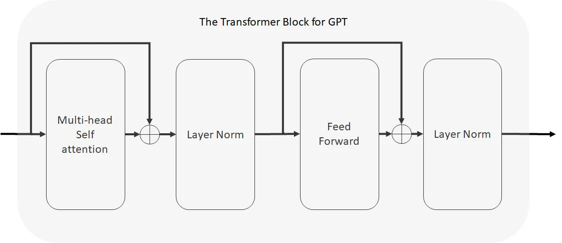
And that’s just about it. It’s known as “transformer” right here as a result of it’s derived from and is a kind of transformer — which is an structure we are going to take a look at within the subsequent part. This doesn’t have an effect on understanding as we’ve already lined all of the constructing blocks proven right here earlier than. Let’s recap every thing we’ve lined to this point constructing as much as this GPT structure:

• We noticed how neural nets take numbers and output different numbers and have weights as parameters which could be educated
• We will connect interpretations to those enter/output numbers and provides actual world that means to a neural community
• We will chain neural networks to create larger ones, and we are able to name every one a “block” and denote it with a field to make diagrams simpler. Every block nonetheless does the identical factor, absorb a bunch of numbers and output different bunch of numbers
• We realized a variety of various kinds of blocks that serve totally different functions
• GPT is only a particular association of those blocks that’s proven above with an interpretation that we mentioned in Half 1

Modifications have been revamped time to this as corporations have constructed as much as highly effective trendy LLMs, however the fundamental stays the identical.

Now, this GPT transformer is definitely what known as a “decoder” within the authentic transformer paper that launched the transformer structure. Let’s check out that.

This is among the key improvements driving speedy acceleration within the capabilities of language fashions not too long ago. Transformers not solely improved the prediction accuracy, they’re additionally simpler/extra environment friendly than earlier fashions (to coach), permitting for bigger mannequin sizes. That is what the GPT structure above relies on.

Should you take a look at GPT structure, you may see that it’s nice for producing the following phrase within the sequence. It basically follows the identical logic we mentioned in Half 1. Begin with just a few phrases after which proceed producing one after the other. However, what when you wished to do translation. What when you had a sentence in german (e.g. “Wo wohnst du?” = “The place do you reside?”) and also you wished to translate it to english. How would we practice the mannequin to do that?

Effectively, very first thing we would want to do is determine a solution to enter german phrases. Which implies now we have to develop our embedding to incorporate each german and english. Now, I assume here’s a merely means of inputting the knowledge. Why don’t we simply concatenate the german sentence firstly of no matter to this point generated english is and feed it to the context. To make it simpler for the mannequin, we are able to add a separator. This may look one thing like this at every step:

This may work, nevertheless it has room for enchancment:

• If the context size is fastened, generally the unique sentence is misplaced
• The mannequin has rather a lot to be taught right here. Two languages concurrently, but additionally to know that <SEP> is the separator token the place it wants to begin translating
• You might be processing your entire german sentence, with totally different offsets, for every phrase era. This implies there will likely be totally different inside representations of the identical factor and the mannequin ought to be capable of work by all of it for translation

Transformer was initially created for this activity and consists of an “encoder” and a “decoder” — that are mainly two separate blocks. One block merely takes the german sentence and offers out an intermediate illustration (once more, bunch of numbers, mainly) — that is known as the encoder.

The second block generates phrases (we’ve seen a variety of this to this point). The one distinction is that along with feeding it the phrases generated to this point we additionally feed it the encoded german (from the encoder block) sentence. In order it’s producing language, it’s context is mainly all of the phrases generated to this point, plus the german. This block known as the decoder.

Every of those encoders and decoders consist of some blocks, notably the eye block sandwiched between different layers. Let’s take a look at the illustration of a transformer from the paper “Consideration is all you want” and attempt to perceive it:

The vertical set of blocks on the left known as the “encoder” and those to the correct known as the “decoder”. Let’s go over and perceive something that now we have not already lined earlier than:

Recap on how one can learn the diagram: Every of the bins here’s a block that takes in some inputs within the type of neurons, and spits out a set of neurons as output that may then both be processed by the following block or interpreted by us. The arrows present the place the output of a block goes. As you may see, we are going to usually take the output of 1 block and feed it in as enter into a number of blocks. Let’s undergo every factor right here:

Feed ahead: A feedforward community is one that doesn’t include cycles. Our authentic community in part 1 is a feed ahead. In-fact, this block makes use of very a lot the identical construction. It incorporates two linear layers, every adopted by a RELU (see observe on RELU in first part) and a dropout layer. Remember the fact that this feedforward neetwork applies to every place independently. What this implies is that the knowledge on place 0 has a feedforward community, and on place 1 has one and so forth.. However the neurons from place x do not need a linkage to the feedforward community of place y. That is essential as a result of if we didn’t do that, it will permit the community to cheat throughout coaching time by wanting ahead.

Cross-attention: You’ll discover that the decoder has a multi-head consideration with arrows coming from the encoder. What’s going on right here? Bear in mind the worth, key, question in self-attention and multi-head consideration? All of them got here from the identical sequence. The question was simply from the final phrase of the sequence in-fact. So what if we stored the question however fetched the worth and key from a totally totally different sequence altogether? That’s what is occurring right here. The worth and key come from the output of the encoder. Nothing has modified mathematically besides the place the inputs for key and worth are coming from now.

Nx: The Nx right here merely represents that this block is chain-repeated N instances. So mainly you’re stacking the block back-to-back and passing the enter from the earlier block to the following one. It is a solution to make the neural community deeper. Now, wanting on the diagram there may be room for confusion about how the encoder output is fed to the decoder. Let’s say N=5. Will we feed the output of every encoder layer to the corresponding decoder layer? No. Principally you run the encoder all over as soon as and solely as soon as. Then you definitely simply take that illustration and feed the identical factor to each one of many 5 decoder layers.

Add & Norm block: That is mainly the identical as beneath (guess the authors had been simply attempting to save lots of house)

Every little thing else has already been mentioned. Now you’ve a whole clarification of the transformer structure build up from easy sum and product operations and absolutely self contained! what each line, each sum, each field and phrase means by way of how one can construct them from scratch. Theoretically, these notes include what you have to code up the transformer from scratch. In-fact, if you’re this repo does that for the GPT structure above.

Matrix Multiplication

We launched vectors and matrices above within the context of embeddings. A matrix has two dimensions (quantity or rows and columns). A vector can be considered a matrix the place one of many dimensions equals one. Product of two matrices is outlined as:

Dots characterize multiplication. Now let’s take a second take a look at the calculation of blue and natural neurons within the very first image. If we write the weights as a matrix and the inputs as vectors, we are able to write the entire operation within the following means:

If the burden matrix known as “W” and the inputs are known as “x” then Wx is the end result (the center layer on this case). We will additionally transpose the 2 and write it as xW — this can be a matter of desire.

Normal deviation

We use the idea of ordinary deviation within the Layer Normalization part. Normal deviation is a statistical measure of how unfold out the values are (in a set of numbers), e.g., if the values are all the identical you’d say the usual deviation is zero. If, on the whole, every worth is de facto removed from the imply of those exact same values, then you’ll have a excessive customary deviation. The method to calculate customary deviation for a set of numbers, a1, a2, a3…. (say N numbers) goes one thing like this: subtract the imply (of those numbers) from every of the numbers, then sq. the reply for every of N numbers. Add up all these numbers after which divide by N. Now take a sq. root of the reply.

Positional Encoding

We talked about positional embedding above. A positional encoding is just a vector of the identical size because the phrase embedding vector, besides it isn’t an embedding within the sense that it isn’t educated. We merely assign a novel vector to each place e.g. a distinct vector for place 1 and totally different one for place 2 and so forth. A easy means of doing that is to make the vector for that place merely filled with the place quantity. So the vector for place 1 could be [1,1,1…1] for two could be [2,2,2…2] and so forth (keep in mind size of every vector should match embedding size for addition to work). That is problematic as a result of we are able to find yourself with giant numbers in vectors which creates challenges throughout coaching. We will, after all, normalize these vectors by dividing each quantity by the max of place, so if there are 3 phrases complete then place 1 is [.33,.33,..,.33] and a pair of is [.67, .67, ..,.67] and so forth. This has the issue now that we’re continuously altering the encoding for place 1 (these numbers will likely be totally different after we feed 4 phrase sentence as enter) and it creates challenges for the community to be taught. So right here, we would like a scheme that allocates a novel vector to every place, and the numbers don’t explode. Principally if the context size is d (i.e., most variety of tokens/phrases that we are able to feed into the community for predicting subsequent token/phrase, see dialogue in “how does all of it generate language?” part) and if the size of the embedding vector is 10 (say), then we want a matrix with 10 rows and d columns the place all of the columns are distinctive and all of the numbers lie between 0 and 1. On condition that there are infinitely many numbers between zero and 1, and the matrix is finitely sized, this may be completed in some ways.

The strategy used within the “Consideration is all you want” paper goes one thing like this:

• Draw 10 sin curves every being si(p) = sin (p/10000(i/d)) (that’s 10k to energy i/d)
• Fill the encoding matrix with numbers such that (i,p)th quantity is si(p), e.g., for place 1 the fifth factor of the encoding vector is s5(1)=sin (1/10000(5/d))

Why select this technique? By altering the ability on 10k you’re altering the amplitude of the sine perform when seen on the p-axis. And if in case you have 10 totally different sine capabilities with 10 totally different amplitudes, then it is going to be a very long time earlier than you get a repetition (i.e. all 10 values are the identical) for altering values of p. And this helps give us distinctive values. Now, the precise paper makes use of each sine and cosine capabilities and the type of encoding is: si(p) = sin (p/10000(i/d)) if i is even and si(p) = cos(p/10000(i/d)) if i is odd.