How Dependable Are Your Predictions?
About
To be thought-about dependable, a mannequin should be calibrated in order that its confidence in every choice intently displays its true consequence. On this weblog submit we’ll check out essentially the most generally used definition for calibration after which dive right into a often used analysis measure for Mannequin Calibration. We’ll then cowl a number of the drawbacks of this measure and the way these surfaced the necessity for added notions of calibration, which require their very own new analysis measures. This submit isn’t supposed to be an in-depth dissection of all works on calibration, nor does it concentrate on the way to calibrate fashions. As an alternative, it’s meant to supply a mild introduction to the completely different notions and their analysis measures in addition to to re-highlight some points with a measure that’s nonetheless extensively used to judge calibration.
Desk of Contents
What’s Calibration?
Calibration makes positive {that a} mannequin’s estimated chances match real-world outcomes. For instance, if a climate forecasting mannequin predicts a 70% probability of rain on a number of days, then roughly 70% of these days ought to truly be wet for the mannequin to be thought-about effectively calibrated. This makes mannequin predictions extra dependable and reliable, which makes calibration related for a lot of functions throughout varied domains.
Now, what calibration means extra exactly is dependent upon the precise definition being thought-about. We’ll take a look at the most typical notion in machine studying (ML) formalised by Guo and termed confidence calibration by Kull. However first, let’s outline a little bit of formal notation for this weblog.
On this weblog submit we think about a classification activity with Okay attainable lessons, with labels Y ∈ {1, …, Okay} and a classification mannequin p̂ :𝕏 → Δᴷ, that takes inputs in 𝕏 (e.g. a picture or textual content) and returns a chance vector as its output. Δᴷ refers back to the Okay-simplex, which simply signifies that the output vector should sum to 1 and that every estimated chance within the vector is between 0 & 1. These particular person chances (or confidences) point out how seemingly an enter belongs to every of the Okay lessons.

1.1 (Confidence) Calibration
A mannequin is taken into account confidence-calibrated if, for all confidences c, the mannequin is appropriate c proportion of the time:

the place (X,Y) is a datapoint and p̂ : 𝕏 → Δᴷ returns a chance vector as its output
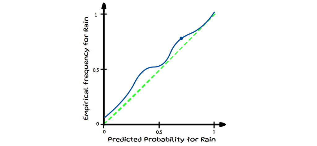
This definition of calibration, ensures that the mannequin’s last predictions align with their noticed accuracy at that confidence stage. The left chart beneath visualises the peerlessly calibrated consequence (inexperienced diagonal line) for all confidences utilizing a binned reliability diagram. On the precise hand facet it reveals two examples for a particular confidence stage throughout 10 samples.
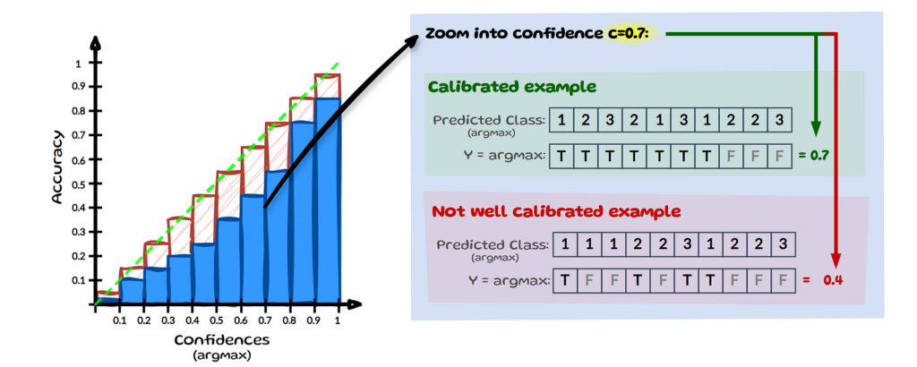
For simplification, we assume that we solely have 3 lessons as in picture 2 (Notation) and we zoom into confidence c=0.7, see picture above. Let’s assume we’ve 10 inputs right here whose most assured prediction (max) equals 0.7. If the mannequin accurately classifies 7 out of 10 predictions (true), it’s thought-about calibrated at confidence stage 0.7. For the mannequin to be absolutely calibrated this has to carry throughout all confidence ranges from 0 to 1. On the similar stage c=0.7, a mannequin could be thought-about miscalibrated if it makes solely 4 appropriate predictions.
2 Evaluating Calibration — Anticipated Calibration Error (ECE)
One extensively used analysis measure for confidence calibration is the Anticipated Calibration Error (ECE). ECE measures how effectively a mannequin’s estimated chances match the noticed chances by taking a weighted common over absolutely the distinction between common accuracy (acc) and common confidence (conf). The measure includes splitting all n datapoints into M equally spaced bins:

the place B is used for representing “bins” and m for the bin quantity, whereas acc and conf are:

ŷᵢ is the mannequin’s predicted class (arg max) for pattern i and yᵢ is the true label for pattern i. 1 is an indicator perform, that means when the anticipated label ŷᵢ equals the true label yᵢ it evaluates to 1, in any other case 0. Let’s have a look at an instance, which can make clear acc, conf and the entire binning method in a visible step-by-step method.
2.1 ECE — Visible Step by Step Instance
Within the picture beneath, we are able to see that we’ve 9 samples listed by i with estimated chances p̂(xᵢ) (simplified as p̂ᵢ) for sophistication cat (C), canine (D) or toad (T). The ultimate column reveals the true class yᵢ and the penultimate column incorporates the anticipated class ŷᵢ.

Solely the utmost chances, which decide the anticipated label are utilized in ECE. Subsequently, we’ll solely bin samples based mostly on the utmost chance throughout lessons (see left desk in beneath picture). To maintain the instance easy we cut up the info into 5 equally spaced bins M=5. If we now have a look at every pattern’s most estimated chance, we are able to group it into one of many 5 bins (see proper facet of picture beneath).

We nonetheless want to find out if the anticipated class is appropriate or not to have the ability to decide the typical accuracy per bin. If the mannequin predicts the category accurately (i.e. yᵢ = ŷᵢ), the prediction is highlighted in inexperienced; incorrect predictions are marked in crimson:

We now have visualised all the knowledge wanted for ECE and can briefly run via the way to
calculate the values for bin 5 (B₅). The opposite bins then merely observe the identical course of, see beneath.

We are able to get the empirical chance of a pattern falling into B₅, by assessing what number of out of all 9 samples fall into B₅, see ( 1 ). We then get the typical accuracy for B₅, see ( 2 ) and lastly the typical estimated chance for B₅, see ( 3 ). Repeat this for all bins and in our small instance of 9 samples we find yourself with an ECE of 0.10445. A superbly calibrated mannequin would have an ECE of 0.
For a extra detailed, step-by-step clarification of the ECE, take a look at this weblog submit.
2.1.1 EXPECTED CALIBRATION ERROR DRAWBACKS
The pictures of binning above present a visible information of how ECE might lead to very completely different values if we used extra bins or maybe binned the identical variety of gadgets as a substitute of utilizing equal bin widths. Such and extra drawbacks of ECE have been highlighted by a number of works early on. Nevertheless, regardless of the recognized weaknesses ECE remains to be extensively used to judge confidence calibration in ML.
3 Most often talked about Drawbacks of ECE
3.1 Pathologies — Low ECE ≠ excessive accuracy
A mannequin which minimises ECE, doesn’t essentially have a excessive accuracy. As an example, if a mannequin at all times predicts the bulk class with that class’s common prevalence because the chance, it is going to have an ECE of 0. That is visualised within the picture above, the place we’ve a dataset with 10 samples, 7 of these are cat, 2 canine and just one is a toad. Now if the mannequin at all times predicts cat with on common 0.7 confidence it will have an ECE of 0. There are extra of such pathologies. To not solely depend on ECE, some researchers use further measures such because the Brier rating or LogLoss alongside ECE.

3.2 Binning Strategy
One of the crucial often talked about points with ECE is its sensitivity to the change in binning. That is generally known as the Bias-Variance trade-off: Fewer bins scale back variance however enhance bias, whereas extra bins result in sparsely populated bins growing variance. If we glance again to our ECE instance with 9 samples and alter the bins from 5 to 10 right here too, we find yourself with the next:

We are able to see that bin 8 and 9 every comprise solely a single pattern and likewise that half the bins now comprise no samples. The above is barely a toy instance, nevertheless since trendy fashions are inclined to have increased confidence values samples usually find yourself in the previous few bins, which suggests they get all the load in ECE, whereas the typical error for the empty bins contributes 0 to ECE.
To mitigate these problems with mounted bin widths some authors have proposed a extra adaptive binning method:

Binning-based analysis with bins containing an equal variety of samples are proven to have decrease bias than a set binning method resembling ECE. This leads Roelofs to induce towards utilizing equal width binning they usually recommend the usage of an alternate: ECEsweep, which maximizes the variety of equal-mass bins whereas guaranteeing the calibration perform stays monotonic. The Adaptive Calibration Error (ACE) and Threshold Adaptive calibration Error (TACE) are two different variations of ECE that use versatile binning. Nevertheless, some discover it delicate to the selection of bins and thresholds, resulting in inconsistencies in rating completely different fashions. Two different approaches intention to get rid of binning altogether: MacroCE does this by averaging over instance-level calibration errors of appropriate and fallacious predictions and the KDE-based ECE does so by changing the bins with non-parametric density estimators, particularly kernel density estimation (KDE).
3.3 Solely most chances thought-about
One other often talked about disadvantage of ECE is that it solely considers the utmost estimated chances. The concept that extra than simply the utmost confidence must be calibrated, is finest illustrated with a easy instance:

Let’s say we educated two completely different fashions and now each want to find out if the identical enter picture incorporates a individual, an animal or no creature. The 2 fashions output vectors with barely completely different estimated chances, however each have the identical most confidence for “no creature”. Since ECE solely appears at these high values it will think about these two outputs to be the identical. But, once we consider real-world functions we would need our self-driving automobile to behave otherwise in a single state of affairs over the opposite. This restriction to the utmost confidence prompted varied authors to rethink the definition of calibration, which provides us two further interpretations of confidence: multi-class and class-wise calibration.
3.3.1 MULTI-CLASS CALIBRATION
A mannequin is taken into account multi-class calibrated if, for any prediction vector q=(q₁,…,qₖ) ∈ Δᴷ, the category proportions amongst all values of X for which a mannequin outputs the identical prediction p̂(X)=q match the values within the prediction vector q.

the place (X,Y) is a datapoint and p̂ : 𝕏 → Δᴷ returns a chance vector as its output
What does this imply in easy phrases? As an alternative of c we now calibrate towards a vector q, with okay lessons. Let’s have a look at an instance beneath:

On the left we’ve the house of all attainable prediction vectors. Let’s zoom into one such vector that our mannequin predicted and say the mannequin has 10 situations for which it predicted the vector q=[0.1,0.2,0.7]. Now to ensure that it to be multi-class calibrated, the distribution of the true (precise) class must match the prediction vector q. The picture above reveals a calibrated instance with [0.1,0.2,0.7] and a not calibrated case with [0.1,0.5,0.4].
3.3.2 CLASS-WISE CALIBRATION
A mannequin is taken into account class-wise calibrated if, for every class okay, all inputs that share an estimated chance p̂ₖ(X) align with the true frequency of sophistication okay when thought-about by itself:

the place (X,Y) is a datapoint; q ∈ Δᴷ and p̂ : 𝕏 → Δᴷ returns a chance vector as its output
Class-wise calibration is a weaker definition than multi-class calibration because it considers every class chance in isolation somewhat than needing the complete vector to align. The picture beneath illustrates this by zooming right into a chance estimate for sophistication 1 particularly: q₁=0.1. But once more, we assume we’ve 10 situations for which the mannequin predicted a chance estimate of 0.1 for sophistication 1. We then have a look at the true class frequency amongst all lessons with q₁=0.1. If the empirical frequency matches q₁ it’s calibrated.

To judge such completely different notions of calibration, some updates are made to ECE to calculate a class-wise error. One thought is to calculate the ECE for every class after which take the typical. Others, introduce the usage of the KS-test for class-wise calibration and likewise recommend utilizing statistical speculation checks as a substitute of ECE based mostly approaches. And different researchers develop a speculation check framework (TCal) to detect whether or not a mannequin is considerably mis-calibrated and construct on this by creating confidence intervals for the L2 ECE.
All of the approaches talked about above share a key assumption: ground-truth labels can be found. Inside this gold-standard mindset a prediction is both true or false. Nevertheless, annotators would possibly unresolvably and justifiably disagree on the actual label. Let’s have a look at a easy instance beneath:

We have now the identical picture as in our entry instance and might see that the chosen label differs between annotators. A standard method to resolving such points within the labelling course of is to make use of some type of aggregation. Let’s say that in our instance the bulk vote is chosen, so we find yourself evaluating how effectively our mannequin is calibrated towards such ‘floor fact’. One would possibly assume, the picture is small and pixelated; after all people is not going to be sure about their selection. Nevertheless, somewhat than being an exception such disagreements are widespread. So, when there may be numerous human disagreement in a dataset it won’t be a good suggestion to calibrate towards an aggregated ‘gold’ label. As an alternative of gold labels increasingly more researchers are utilizing gentle or clean labels that are extra consultant of the human uncertainty, see instance beneath:

In the identical instance as above, as a substitute of aggregating the annotator votes we might merely use their frequencies to create a distribution Pᵥₒₜₑ over the labels as a substitute, which is then our new yᵢ. This shift in the direction of coaching fashions on collective annotator views, somewhat than counting on a single source-of-truth motivates one other definition of calibration: calibrating the mannequin towards human uncertainty.
3.3.3 HUMAN UNCERTAINTY CALIBRATION
A mannequin is taken into account human-uncertainty calibrated if, for every particular pattern x, the anticipated chance for every class okay matches the ‘precise’ chance Pᵥₒₜₑ of that class being appropriate.

the place (X,Y) is a datapoint and p̂ : 𝕏 → Δᴷ returns a chance vector as its output.
This interpretation of calibration aligns the mannequin’s prediction with human uncertainty, which suggests every prediction made by the mannequin is individually dependable and matches human-level uncertainty for that occasion. Let’s take a look at an instance beneath:

We have now our pattern information (left) and zoom right into a single pattern x with index i=1. The mannequin’s predicted chance vector for this pattern is [0.1,0.2,0.7]. If the human labelled distribution yᵢ matches this predicted vector then this pattern is taken into account calibrated.
This definition of calibration is extra granular and strict than the earlier ones because it applies straight on the stage of particular person predictions somewhat than being averaged or assessed over a set of samples. It additionally depends closely on having an correct estimate of the human judgement distribution, which requires a lot of annotations per merchandise. Datasets with such properties of annotations are regularly turning into extra out there.
To judge human uncertainty calibration the researchers introduce three new measures: the Human Entropy Calibration Error (EntCE), the Human Rating Calibration Rating (RankCS) and the Human Distribution Calibration Error (DistCE).

the place H(.) signifies entropy.
EntCE goals to seize the settlement between the mannequin’s uncertainty H(p̂ᵢ) and the human uncertainty H(yᵢ) for a pattern i. Nevertheless, entropy is invariant to the permutations of the chance values; in different phrases it doesn’t change while you rearrange the chance values. That is visualised within the picture beneath:

On the left, we are able to see the human label distribution yᵢ, on the precise are two completely different mannequin predictions for that very same pattern. All three distributions would have the identical entropy, so evaluating them would lead to 0 EntCE. Whereas this isn’t excellent for evaluating distributions, entropy remains to be useful in assessing the noise stage of label distributions.

the place argsort merely returns the indices that might kind an array.
So, RankCS checks if the sorted order of estimated chances p̂ᵢ matches the sorted order of yᵢ for every pattern. In the event that they match for a specific pattern i one can rely it as 1; if not, it may be counted as 0, which is then used to common over all samples N.¹
Since this method makes use of rating it doesn’t care in regards to the precise measurement of the chance values. The 2 predictions beneath, whereas not the identical in school chances would have the identical rating. That is useful in assessing the general rating functionality of fashions and appears past simply the utmost confidence. On the similar time although, it doesn’t absolutely seize human uncertainty calibration because it ignores the precise chance values.


DistCE has been proposed as an extra analysis for this notion of calibration. It merely makes use of the whole variation distance (TVD) between the 2 distributions, which goals to mirror how a lot they diverge from each other. DistCE and EntCE seize occasion stage data. So to get a sense for the complete dataset one can merely take the typical anticipated worth over absolutely the worth of every measure: E[∣DistCE∣] and E[∣EntCE∣]. Maybe future efforts will introduce additional measures that mix the advantages of rating and noise estimation for this notion of calibration.
4 Remaining ideas
We have now run via the most typical definition of calibration, the shortcomings of ECE and the way a number of new notions of calibration exist. We additionally touched on a number of the newly proposed analysis measures and their shortcomings. Regardless of a number of works arguing towards the usage of ECE for evaluating calibration, it stays extensively used. The intention of this weblog submit is to attract consideration to those works and their different approaches. Figuring out which notion of calibration most closely fits a particular context and the way to consider it ought to keep away from deceptive outcomes. Possibly, nevertheless, ECE is solely really easy, intuitive and simply ok for many functions that it’s right here to remain?

Within the meantime, you’ll be able to cite/reference the ArXiv preprint.
Footnotes
¹Within the paper it’s acknowledged extra typically: If the argsorts match, it means the rating is aligned, contributing to the general RankCS rating.